Solving Schrödinger's Equation in 1,2,3-D with MATLAB
In my junior year, I picked an elective on Quantum Mechanics: Electronic Devices. The project that was worth 50% was to solve the time-independent Schrodinger's equation in 1,2,3-D numerically, using MATLAB.
I already had a fascination for modern physics. Therefore, I spent disproportionately more time on this project. I researched a lot, learned about numerical methods and the intuition of Schrodinger's Equation.
Through this, I understood Schrodinger's equation in two levels:
- Mathematically, it is a simple-harmonic-motion in space. I was fascinated to find that in 3-D, with a point charge, this SHM yields the s-p-d orbitals of the hydrogen atom. Later I found that such 'harmonic oscillators' are found at the foundations of different branches of physics.
- It basically says that wavefunctions are the eigenfunctions and the discrete energy values are the eigenvalues of the Hamiltonian operator, which is constrained by the potential field.

Although I learned eigen-things in Linear Algebra class, I did not have an intuition for them. Therefore, I spent a few days building up a deeper intuition about them. I watched this entire series, took copious notes.
I then started programming using some references. While we were asked only to do it for either 1,2 or 3D using any method, I went the extra mile and did it for all three, using two methods.
For better intuition on wavefunctions and observables of Quantum Mechanics, check out my following post:
 Abarajithan G
Report
The intuition I gained from this, led me to write this explanation of basic QM, and this rant about how Linear Algebra is introduced poorly.
MATLAB Code
Two of the five Matlab programs I wrote are given here for reference.
Solving 1D equation directly
clear all
close all
clc

% Parameters
n=4;
Nx = 200;
Lmax = 4e-8;

% Constants
h =6.626E-34;
hbar =h/(2*pi);
e =1.602E-19;
me =9.109E-31;


% Potential
x = linspace(0,Lmax, Nx);
V = 0.3*[ones(1,50) zeros(1,100) ones(1,50)];
%V = 0.01*sin(1E11*pi*x);

%% Direct Method
dx=x(2)-x(1);

% Build Laplacian
DX2 = (-2)*diag(ones(1,Nx)) + (1)*diag(ones(1,Nx-1),-1) + (1)*diag(ones(1,Nx-1),1);
DX2 = DX2/dx^2;

% Build Hamiltonian
H = -hbar^2/(2*me) * DX2  +  diag(V*e);

% Solve for Eigenfunction
H = sparse(H);
[psi,Energy] = eigs(H,n,'SM');
E = diag(Energy)/e ;      %Divide by e for eV units
E = abs(E);

% Normalize Wavefunction
for i=1:n
    psi(:,i)=psi(:,i)/sqrt(trapz(x',abs(psi(:,i)).^2));
end

psi=psi(:,end:-1:1);
E=E(end:-1:1);

%% Plot Results

% Normalise for plotting
for i=1:length(E)
      psi(:,i)=abs(psi(:,i)).^2/max(abs(psi(:,i)).^2)*0.04 + E(i)*15;
end

LW=2;
figure
for i=1:length(E)

    plot(x*1e9,V, 'b-','linewidth',LW)
    hold on;
    plot(x*1e9,psi(:,i),'r-','linewidth',LW)

    xlabel('x (nm)');
    ylabel('Energy (eV)');

    ylim([min(V)-0.05 max(V)+0.1])
    hold on;
end
hold off;
Solving 3D equation in fourier domain
clear all
close all
clc
% Constants
h=6.62606896E-34;
hbar=h/(2*pi);
e=1.602176487E-19;
me=9.10938188E-31;
ep0 = 8.854E-12;
n=12;
Nx=64;
Ny=64;
Nz=64;
Mass = 0.23;
Mx=15e-9;
My=15e-9;
Mz=4e-9;
x=linspace(-Mx/2,Mx/2,Nx);
y=linspace(-My/2,My/2,Ny);
z=linspace(-Mz,Mz,Nz)+0.5e-9;
[X,Y,Z]=meshgrid(x,y,z);
%% Define Potential
% V=1.5;
% V0 = (1-index) * V;
% 1. Rectangular potential well
%index = (X > -Mx*0.4) .* (X < Mx*0.4) .* (Y > -My*0.4) .* (Y < My*0.4).* (Z > -Mz*0.4) .* (Z < Mz*0.4);
% 2. Circular potential well
%index = (X.^2 + Y.^2 + Z.^2) < (Mx*0.4)^2;
% 3. Point charge - hydrogen atom
V0 = (1/(4*pi*ep0))*(1-e/(sqrt(X.^2+Y.^2+Z.^2)));
%% Fourier Method
Nx = 64 ;
Ny = 64 ;
Nz = 64 ;
NGx = 15;
NGy = 13;
NGz = 11;
% Building the fourier space
NGx = 2*floor(NGx/2);
NGy = 2*floor(NGy/2);
NGz = 2*floor(NGz/2);
[X,Y,Z] = meshgrid(x,y,z);
xx=linspace(x(1),x(end),Nx);
yy=linspace(y(1),y(end),Ny);
zz=linspace(z(1),z(end),Nz);
[XX,YY,ZZ] = meshgrid(xx,yy,zz);
V=interp3(X,Y,Z,V0,XX,YY,ZZ);
dx=x(2)-x(1);
dxx=xx(2)-xx(1);
dy=y(2)-y(1);
dyy=yy(2)-yy(1);
dz=z(2)-z(1);
dzz=zz(2)-zz(1);
Ltotx=xx(end)-xx(1);
Ltoty=yy(end)-yy(1);
Ltotz=zz(end)-zz(1);
[XX,YY,ZZ] = meshgrid(xx,yy,zz);
% Potential function in Fourier space
Vk = fftshift(fftn(V))*dxx*dyy*dzz/Ltotx/Ltoty/Ltotz;
Vk =Vk(Ny/2-NGy+1:Ny/2+NGy+1 , Nx/2-NGx+1:Nx/2+NGx+1 , Nz/2-NGz+1:Nz/2+NGz+1);
% k vectors
Gx = (-NGx/2:NGx/2)'*2*pi/Ltotx;
Gy = (-NGy/2:NGy/2)'*2*pi/Ltoty;
Gz = (-NGz/2:NGz/2)'*2*pi/Ltotz;
NGx=length(Gx);
NGy=length(Gy);
NGz=length(Gz);
NG=NGx*NGy*NGz;
% Building Hamiltonian
idx_x = reshape(1:NGx, [1 NGx 1]);
idx_x = repmat(idx_x, [NGy 1 NGz]);
idx_x = idx_x(:);
idx_y = reshape(1:NGy, [NGy 1 1]);
idx_y = repmat(idx_y, [1 NGx NGz]);
idx_y = idx_y(:);
idx_z = reshape(1:NGz, [1 1 NGz]);
idx_z = repmat(idx_z, [NGy NGx 1]);
idx_z = idx_z(:);
idx_X = (repmat(idx_x,[1 NG])-repmat(idx_x',[NG 1])) + NGx;
idx_Y = (repmat(idx_y,[1 NG])-repmat(idx_y',[NG 1])) + NGy;
idx_Z = (repmat(idx_z,[1 NG])-repmat(idx_z',[NG 1])) + NGz;
idx = sub2ind(size(Vk), idx_Y(:), idx_X(:), idx_Z(:));
idx = reshape(idx, [NG NG]);
GX = diag(Gx(idx_x));
GY = diag(Gy(idx_y));
GZ = diag(Gz(idx_z));
D2 = GX.^2 + GY.^2 + GZ.^2 ;
H = hbar^2/(2*me*Mass)*D2 + Vk(idx)*e ;
% Solving for eigs
H = sparse(H);
[psik, Ek] = eigs(H,n,'SM');
E = diag(Ek) / e;
E=real(E);
% Invert and normalize wavefunctions
for j=1:n
PSI = reshape(psik(:,j),[NGy,NGx,NGz]);
% Inverse FT
Nkx=length(PSI(1,:,1));
Nky=length(PSI(:,1,1));
Nkz=length(PSI(1,1,:));
Nx1=Nx/2-floor(Nkx/2);
Nx2=Nx/2+ceil(Nkx/2);
Ny1=Ny/2-floor(Nky/2);
Ny2=Ny/2+ceil(Nky/2);
Nz1=Nz/2-floor(Nkz/2);
Nz2=Nz/2+ceil(Nkz/2);
PSI00=zeros(Ny,Nx,Nz);
PSI00( Ny1+1:Ny2 , Nx1+1:Nx2 , Nz1+1:Nz2)=PSI;
PSI=ifftn(ifftshift(PSI00));
PSI = PSI/(dxx*dyy*dzz) ;
psi_temp = interp3(XX,YY,ZZ,PSI,X,Y,Z);
psi(:,:,:,j) = psi_temp / max(psi_temp(:));
end
%% Plot results
c=0;
ii=0;
for i=1:n
if i>18
break
end
if i==1 || i==5 || i==9 || i == 13
figure
c=c+1;
ii=0;
end
ii=ii+1;
subplot(2,2,ii,'fontsize',10)
hold on;grid on;view (-38, 20);
idz=find(z>0);idz=idz(1);
pcolor(x*1e9,y*1e9,squeeze(V0(:,:,idz)))
colormap(jet)
PSI=abs(psi(:,:,:,i)).^2;
p = patch(isosurface(x*1e9,y*1e9,z*1e9,PSI,max(PSI(:))/6));
isonormals(x*1e9,y*1e9,z*1e9,PSI, p)
set(p, 'FaceColor', 'blue', 'EdgeColor', 'none', 'FaceLighting', 'gouraud')
daspect([1,1,1])
light ('Position', [1 1 5]);
M=max([Mx My]);
xlim([-1 1]*M/3*1e9)
ylim([-1 1]*M/3*1e9)
zlim([-1 1]*M/3*1e9)
xlabel('x (nm)')
ylabel('y (nm)')
zlabel('z (nm)')
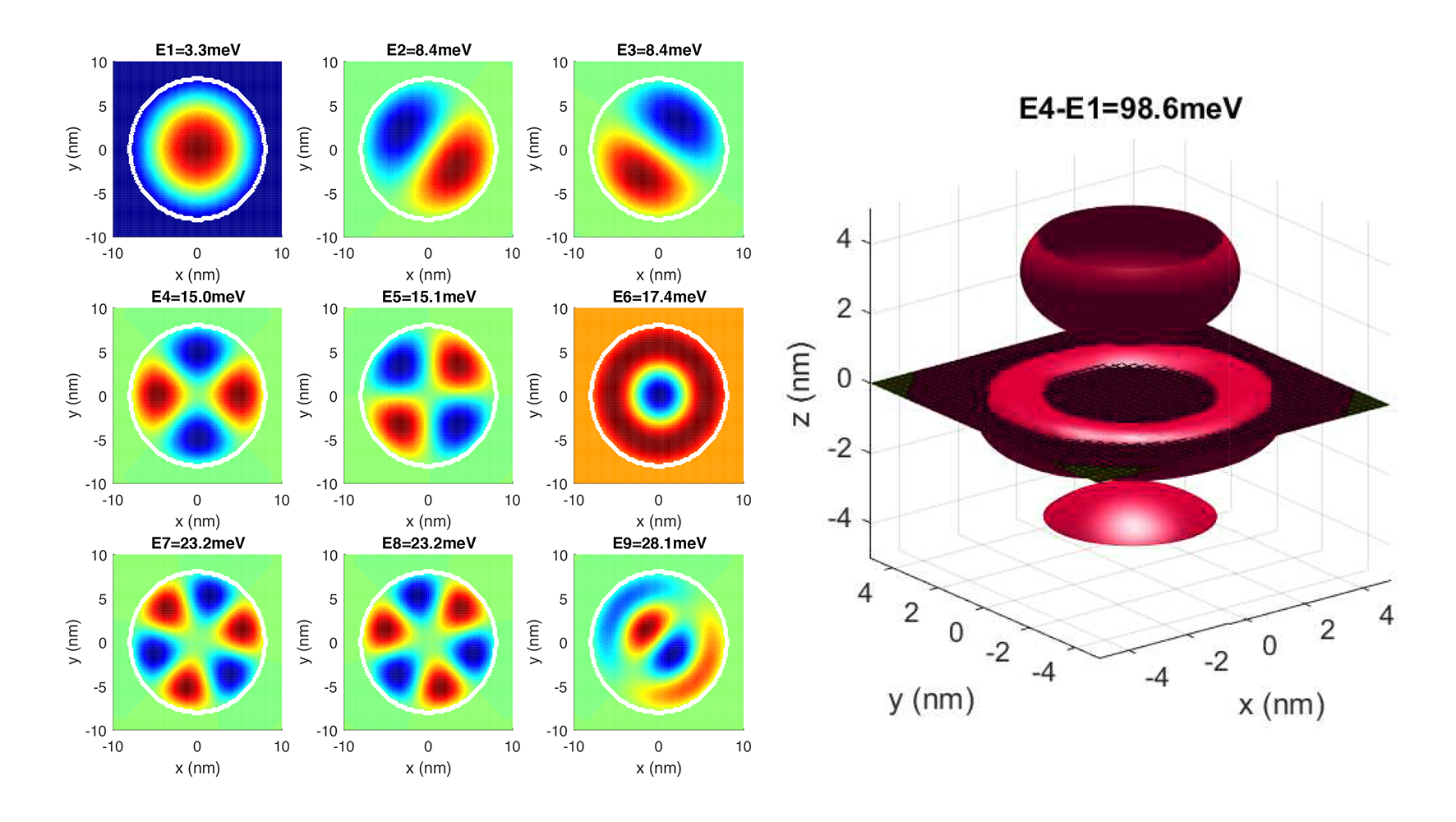
title(strcat('E',num2str(i),'-E1=',num2str((E(i)-E(1))*1000,'%.1f'),'meV'))
endReferences
- [1] “(17) A Numerical Approach to the Solution of Schrodinger Equation for Hydrogen-Like Atoms | Request PDF,” ResearchGate. [Online]. Available: https://www.researchgate.net/publication/305818710_A_Numerical_Approach_to_the_Solution_of_Schrodinger_Equation_for_Hydrogen-Like_Atoms.
- [2] LaurentNevou, 3D Time independent Schroedinger equation solver. Contribute to LaurentNevou/Q_Schrodinger3D_demo development by creating an account on GitHub. 2019.
- [3] M. A. Mahmood, “A Numerical Approach to the Solution of Schrodinger Equation for Hydrogen-Like Atoms,” IOSR Journal of Dental and Medical Sciences, vol. 15, no. 07, pp. 128–131, Jul. 2016.
- [5] S. P. Novikov, “Discrete Schrodinger operators and topology,” arXiv:math-ph/9903025, Mar. 1999.
- [6] I. Cooper, “DOING PHYSICS WITH MATLAB QUANTUM PHYSICS HYDROGEN ATOM HYDROGEN-LIKE IONS,” p. 40.
- [7] I. Cooper, “DOING PHYSICS WITH MATLAB QUANTUM PHYSICS SCHRODINGER EQUATION,” p. 7.
- [9] “Fourier Transforms of the Time Independent Schroedinger Equation.” [Online]. Available: http://www.sjsu.edu/faculty/watkins/schrofourier.htm.
- [10] “Generate sparse matrix for the Laplacian differential operator ∇2u for 3D grid.” [Online]. Available: https://www.12000.org/my_notes/mma_matlab_control/KERNEL/KEse83.htm
- [12] “LAPLACIAN - The Discrete Laplacian Operator.” [Online]. Available: https://people.sc.fsu.edu/~jburkardt/m_src/laplacian/laplacian.html.
- [13] M. A. Mahmood, “Novel Numerical Solution of Schrodinger Equation for Hydrogen-like Atoms,” vol. 6, no. 3, p. 5, 2015.
- [14] G. Lindblad, “Quantum Mechanics with MATLAB,” p. 28.